作者简介：热爱科研的Matlab仿真开发者，修心和技术同步精进，matlab项目合作可私信。

个人主页：Matlab科研工作室

个人信条：格物致知。

更多Matlab仿真内容点击

智能优化算法       神经网络预测       雷达通信      无线传感器        电力系统

信号处理              图像处理               路径规划       元胞自动机        无人机

内容介绍

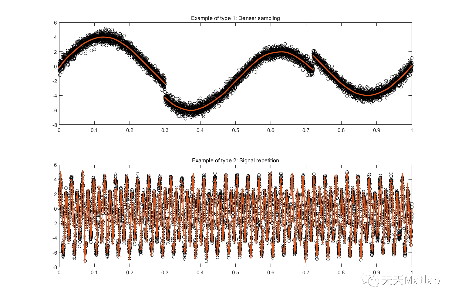
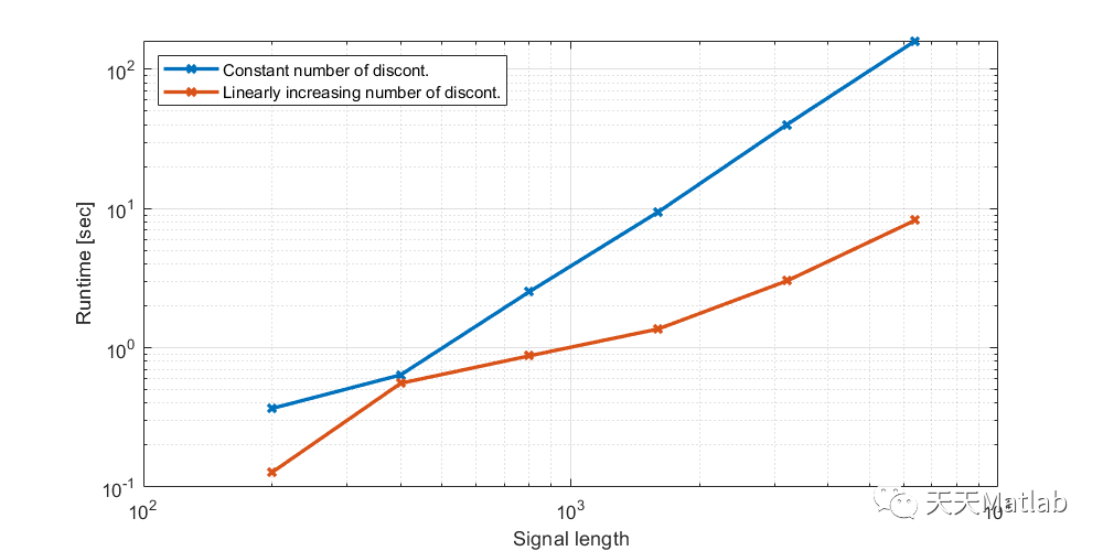
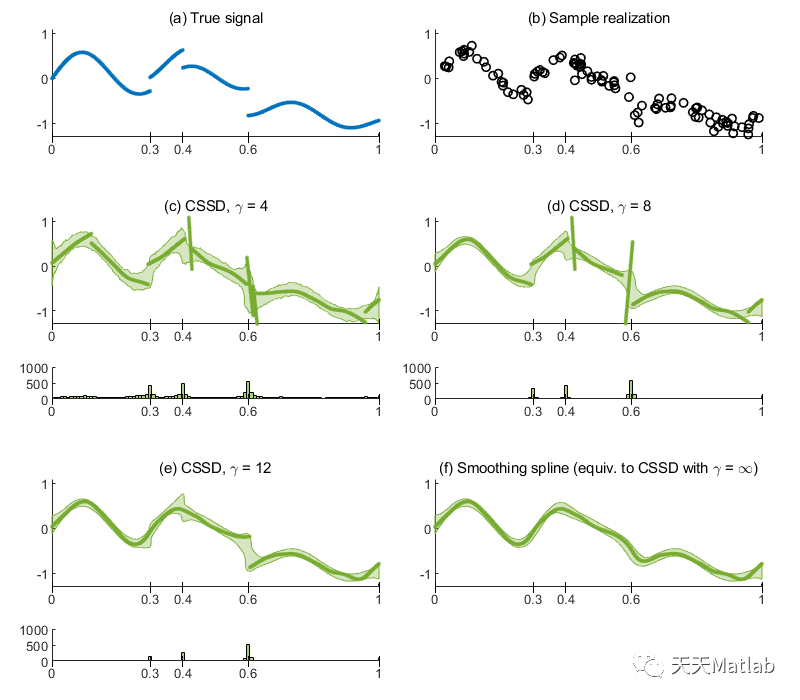
Smoothing splines are standard methods of nonparametric regression for obtaining smooth functions from noisy observations. But as splines are twice differentiable by construction, they cannot capture potential discontinuities in the underlying signal. The smoothing spline model can be augmented such that discontinuities at a priori unknown locations are incorporated. The augmented model results in a minimization problem with respect to discontinuity locations. The minimizing solution is a cubic smoothing spline with discontinuities (CSSD) which may serve as function estimator for discontinuous signals, as a changepoint detector, and as a tool for exploratory data analysis. However, these applications are hardly accessible at the moment because there is no efficient algorithm for computing a CSSD. In this paper, we propose an efficient algorithm that computes a global minimizer of the underlying problem. Its worst case complexity is quadratic in the number of data points. If the number of detected discontinuities scales linearly with the signal length, we observe linear growth of the runtime. By the proposed algorithm, a CSSD can be computed in reasonable time on standard hardware. Furthermore, we implement a strategy for automatic selection of the hyperparameters. Numerical examples demonstrate the applicability of a CSSD for the tasks mentioned above.

部分代码

function output = cssd_cv(x, y, folds_cell, delta, startingPoint, varargin)%CSSD_CV K-Fold cross validation for cubic smoothing spline with discontinuities %% cssd_cv(x, y, folds_cell, delt, xx, delta) automatically determines% the model parameters p and gamma of a CSSD model based on minimization of % a K-fold cross validation score. % % Note: The minimization process uses standard derivative free% optimizers (simulated annealing and Nelder-Mead simplex downhill). So it% is not guaranteed that the result is a global minimum. % Trying different starting points often helps if the results with the default starting point % are unsatisfactory.%% Input% x: vector of data sites%% y: vector of same lenght as x or matrix where y(:,i) is a data vector at site x(i)%% folds_cell (optional): a cell array of index vectors corresponding to the% K folds (if [] the 5 folds are chosen randomly)% % startingPoint (optional): Starting point startingPoint = [p; gamma] for the optimizer% (default is [0.5; 1])%% delta: (optional) weights of the data sites. delta may be thought of as the% standard deviation of the at site x_i. Should have the same size as x.% - Note: The Matlab built in spline function csaps uses a different weight% convention (w). delta is related to Matlab's w by w = 1./delta.^2% - Note for vector-valued data: Weights are assumed to be identical over% vector-components. (Componentwise weights might be supported in a future version.)%% Output% output = cssd_cv(...)% output.p: % p: parameter between 0 and 1 that weights the rougness penalty% (high values result in smoother curves)% output.gamma: parameter between 0 and Infinity that weights the discontiuity% penalty (high values result in less discontinuities, gamma = Inf corresponds to a classical smoothing spline% output.cv_score: best cv_score achieved by the optimizer% output.cv_fun: a function handle to the CV scoring function%% See also CSSDif nargin < 3 folds_cell = {};endif nargin < 4 delta = [];endif nargin < 5 startingPoint = [];endp = inputParser;addOptional(p,'verbose', 0);addOptional(p,'maxTime', Inf);parse(p,varargin{:});verbose = p.Results.verbose;maxTime = p.Results.maxTime;if isempty(delta) delta = ones(size(x));end% checks arguments and creates column vectors (chckxywp is Matlab built in)% Matlab uses the parameter w which is related to delta of De Boor's book by w = 1./delta.^2w = 1./delta.^2;[xi,yi,~,wi] = chckxywp(x,y,2,w,0);deltai = sqrt(1./wi);[N,D] = size(yi);% create folds if not givenif isempty(folds_cell) folds_cell = kfoldcv_split(N, 5);endgamma_tf = @(b) atan(b) * 2/pi;gamma_itf = @(a) (tan(a * pi/2));% generate cv score functioncv_fun = @(p, gamma) cssd_cvscore(xi, yi, p, gamma, deltai, folds_cell);cv_fun_vec = @(z) cv_fun(z(1), gamma_itf(z(2))); % vectorised and transformed version for optimization% perform optimizationsaoptions = {@simulannealbnd,'MaxTime', maxTime};options = {};if verbose saoptions = {saoptions{:}, 'Display','iter','PlotFcns', {@saplotbestx,@saplotbestf,@saplotx,@saplotf}}; options = {options{:}, 'Display','iter', 'PlotFcns', {@optimplotx, @optimplotfunccount, @optimplotfval}};end% set starting point of optimizersif isempty(startingPoint) startingPoint = [0.5; 1]; % starting values: p =0.5, gamma = 1end% transform starting point to lie in the unit square [0,1]^2startingPoint_tf = [startingPoint(1); gamma_tf(startingPoint(2))];% invoke chain of standard derivative-free optimizers on [0,1]^2: simulated% annealing followed by Nelder-Mead simplex downhill[improvedPoint_tf, cv_score] = simulannealbnd(cv_fun_vec, startingPoint_tf, [0;0], [1;1], optimoptions(saoptions{:})); % simulated annealing[improvedPoint_tf, cv_score] = fminsearch(cv_fun_vec, improvedPoint_tf, optimset(options{:})); % refine result of simulated annealing by Nelder Mead downhill% improved p and gammap = improvedPoint_tf(1);gamma = gamma_itf(improvedPoint_tf(2)); % transform gamma back to [0, Inf)% set ouptputoutput.p = p;output.gamma = gamma;output.cv_score = cv_score;output.cv_fun = cv_fun;end

运行结果

参考文献

M. Storath, A. Weinmann, "Smoothing splines for discontinuous signals", arXiv:2211.12785, 2022

️ 代码获取关注我

️部分理论引用网络文献，若有侵权联系博主删除

️ 关注我领取海量matlab电子书和数学建模资料

仿真咨询

1.卷积神经网络（CNN）、LSTM、支持向量机（SVM）、最小二乘支持向量机（LSSVM）、极限学习机（ELM）、核极限学习机（KELM）、BP、RBF、宽度学习、DBN、RF、RBF、DELM实现风电预测、光伏预测、电池寿命预测、辐射源识别、交通流预测、负荷预测、股价预测、PM2.5浓度预测、电池健康状态预测、水体光学参数反演、NLOS信号识别、地铁停车精准预测、变压器故障诊断

2.图像识别、图像分割、图像检测、图像隐藏、图像配准、图像拼接、图像融合、图像增强、图像压缩感知

3.旅行商问题（TSP）、车辆路径问题（VRP、MVRP、CVRP、VRPTW等）、无人机三维路径规划、无人机协同、无人机编队、机器人路径规划、栅格地图路径规划、多式联运运输问题、车辆协同无人机路径规划

4.无人机路径规划、无人机控制、无人机编队、无人机协同、无人机任务分配

5.传感器部署优化、通信协议优化、路由优化、目标定位

6.信号识别、信号加密、信号去噪、信号增强、雷达信号处理、信号水印嵌入提取、肌电信号、脑电信号

7.生产调度、经济调度、装配线调度、充电优化、车间调度、发车优化、水库调度、三维装箱、物流选址、货位优化

8.微电网优化、无功优化、配电网重构、储能配置

9.元胞自动机交通流 人群疏散 病毒扩散 晶体生长